
Check the complete measurement system
Modern potentiostats must be operated under conditions appropriate to the cell and signal being studied. Instrument accuracy alone is not the uncertainty of the complete experiment.
Electrochemical techniques are sensitive to experimental errors. Setup, connections and cell geometry jointly influence measurement quality. This revised archive guide retains the original topics while qualifying broad claims. Original manufacturer background.
Shielding and interference sources
Mains interference and nearby instruments can affect results. A Faraday cage may help with low currents or high impedances; the original 10 µA example is not a universal threshold. Connect the cage to the appropriate ground or shielding point according to the instrument instructions. Adding an arbitrary extra ground connection can create a ground loop.
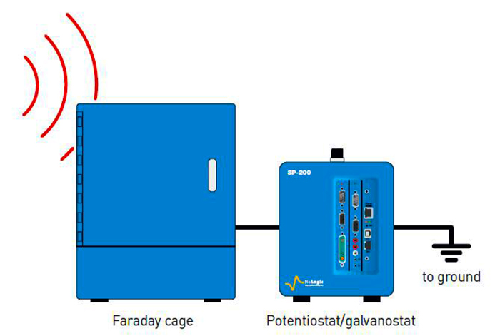
Our suggested troubleshooting check compares the cell signal with a known dummy load at identical settings, then examines nearby interference sources one at a time. This helps locate a problem; it does not replace calibration.
Averaging: which noise decreases?
For independent, equal-variance, zero-mean random errors, the standard deviation of an average of N samples is σ/√N. Four samples then halve it. Drift, correlated noise or systematic error need not follow that improvement. The averaging window can also smooth genuine rapid changes.
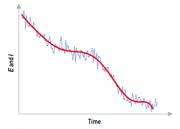
Our numerical example: independent noise with an 8 nA standard deviation would fall to 2 nA when averaging 16 samples. An additional constant 5 nA offset would remain. These are illustrative calculations, not an instrument noise specification.
Filtering and time resolution
A low-pass filter attenuates higher-frequency components; it does not perfectly remove every component above a cutoff. It can change amplitude and phase and introduce delay. Hardware filtering and post-processing sampled data are not interchangeable in every respect.
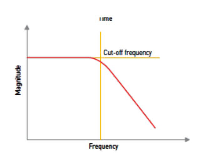
The original EC-Lab setting advice refers to a historical interface. Check available filters and cutoffs for the actual instrument and software version. Keep raw data and document averaging, sampling, analogue and digital filtering. Filtering cannot recover information lost during acquisition.
Reference-electrode condition
High reference impedance together with input and cable capacitances can distort high-frequency EIS. The original 1 kΩ and MHz example is not a universal acceptance limit. Check filling solution, junction, potential stability and manufacturer instructions.
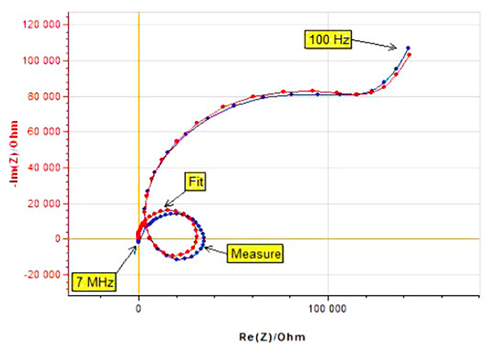
Our reference-electrode guide distinguishes potential-drift checks from impedance checks.
Two-wire and four-point measurements
Four-point, Kelvin-style connections separate current-carrying and voltage-sensing leads. Ideally, negligible current flows through the high-impedance sensing input, excluding voltage drops in current leads outside the sense points. Their location matters: contacts and materials between those points still contribute to the measured voltage.
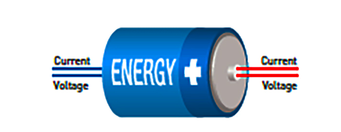
Our ideal example uses 2 A and 20 mΩ total lead resistance outside the sense points, which would add 40 mV in a two-wire measurement. Correctly positioned separate voltage sensing can exclude this term; it does not remove polarisation inside the cell.
Inductance and wiring
Inductive voltage is U = L·dI/dt: current-change rate matters as well as magnitude. In EIS the contribution is frequency-dependent. Distortion does not always imply a larger real resistance, and there is no universal 10 A threshold.
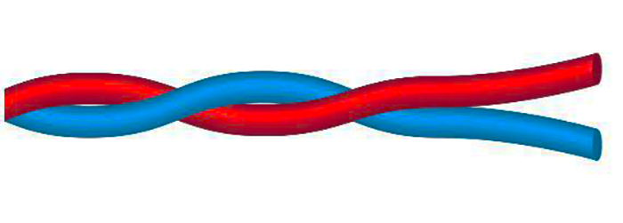
Keep loop area small and wiring repeatable; apply twisting and shielding according to manufacturer instructions. Extensions can add resistance and parasitic elements. In our example, 1 µH at 1 A/ms gives 1 mV. Instrument bandwidth and measurement timing determine how this appears in the recorded data.
Cell geometry and iR drop
Ions carry current through the electrolyte. Solution resistance can make the measured electrode potential differ from that at the reaction surface. With positive anodic current and a simple uncompensated-resistance model, E_surface(t) = E_measured(t) − I(t)Rᵤ. For a linear programme E_measured = Eᵢ + vt; do not confuse that programme with the corrected surface potential in the original equation.
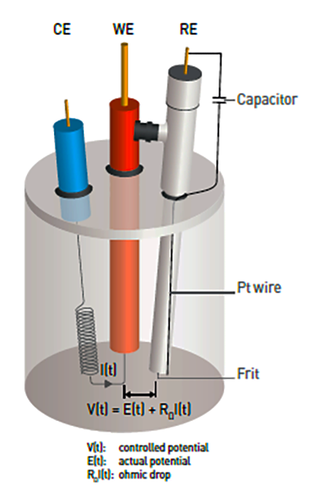
This is a historical connection example, not a universal wiring recipe. Reference position and cell geometry affect uncompensated resistance. Our iR-compensation guide explains correction signs and limits.
Specifications: range and accuracy
For DC measurements, check minimum and maximum expected current, the potential window, compliance limit and range-dependent error together. Displayed decimal places do not establish low uncertainty.
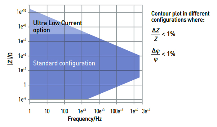
For EIS, excitation, cables and configuration matter alongside frequency and impedance. Read contour diagrams with their specified test conditions; the historical figure is not an accuracy map for every current instrument. See the EIS data-quality guide.
Documentation and further reading
A manufacturer PDF of the laboratory-practices poster is available, replacing the archive’s missing-poster notice. The locally retained metrology tutorial is also available; treat its instrument and software examples as historical.
- AN27: effects of ohmic drop.
- AN28: resistance-measurement methods and AN29: ZIR.
- AN44: EIS artefacts and AN48: corrosion analysis.
- TN13: long cell cables. Locate the older TN15 through manufacturer support by its title, Low current option: measurement precautions.
Retain configuration, wiring, cell state, software version and processing steps together. This makes differences between repeated measurements easier to interpret.