Introduction
Historical instrument examples: VMP-3, BCS-815 and the older BT-Lab screenshots are retained from the original article. Check the current instrument catalogue and the actual configuration for present capabilities and options.
Lithium-ion battery development has expanded with portable electronics and electric vehicles. Reliable testing is necessary for development and quality control. Multiple channels and automated analysis support parallel experiments, but actual channel count, functions and accuracy depend on the configuration.
Electrochemical methods complement cycling with further information. State or lifetime estimation requires suitable data quality, a validated model and representative tests; software does not automatically provide a certain prognosis. Understanding both methods and limitations matters in research, integration and servicing.
This article introduces the equipment, software workflows and methods used to investigate lithium-ion cells.
Why test batteries?
Battery applications are diverse, so the measurements must address the intended use.

Useful questions include:
- What is the state of charge (SoC)?
- How has the cell changed from its initial condition, or state of health (SoH)?
- What capacity is available under the intended protocol?
- Which charge and discharge limits apply to this cell?
- How does it behave under realistic load and charge fluctuations?
- Which cells constrain a module’s performance?
Results must be sufficiently accurate and repeatable for the decision. Test conditions should represent practical operation, while controlled comparison experiments may intentionally isolate individual influences.
Who needs which tests?
Cell manufacturers, module builders and equipment integrators have different testing priorities. Manufacturing quality control examines conformity; integrators need evidence that the selected cells meet their product requirements.
Matching cells matters in series or parallel groups. Capacity, resistance and state differences can limit a module, although the exact constraint depends on its architecture and management system. Screening criteria must therefore follow the intended application rather than a universal “good cell” label. Equipment manufacturers using purchased cells or building modules need tests suited to their products: an unsuitable supply can undermine the performance of the complete instrument. Where matching is required, compare individual cells under the same conditions and select against defined tolerances. A quick screening result need not describe every aspect of long-term behaviour.
Standby use requires sufficient available charge and verified readiness. Cyclic use involves repeated charge and discharge, often under variable load: handling equipment, cleaning machines and tools are examples. Application or “urban” profiles represent this variability. Standby systems may need a controlled recharge when available charge is insufficient, especially where continuous maintenance charging is not used. The charging decision must follow the cell and system instructions rather than a generic rule.
Basic parameters
Cell voltage is the instantaneous potential difference between the terminals. It changes with operating state and carries information about the electrochemical processes.
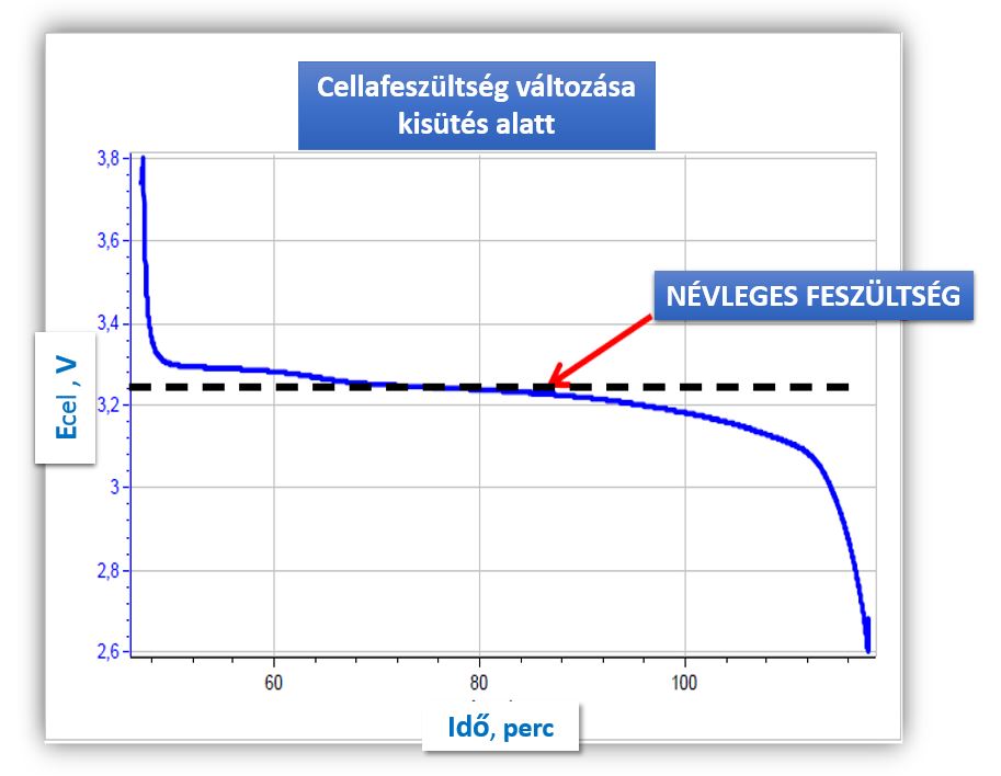
The voltage of a series group is the sum of cell voltages. Multiplying one cell voltage by cell count is valid when those voltages are equal. Nominal voltage is a designated representative value, not the instantaneous terminal voltage.
Capacity is charge available under a specified protocol, commonly in Ah: 1 Ah = 3600 C. It is not energy. Current, temperature and voltage limits affect the result. Q = ∫I(t)dt, or IΔt at constant current.
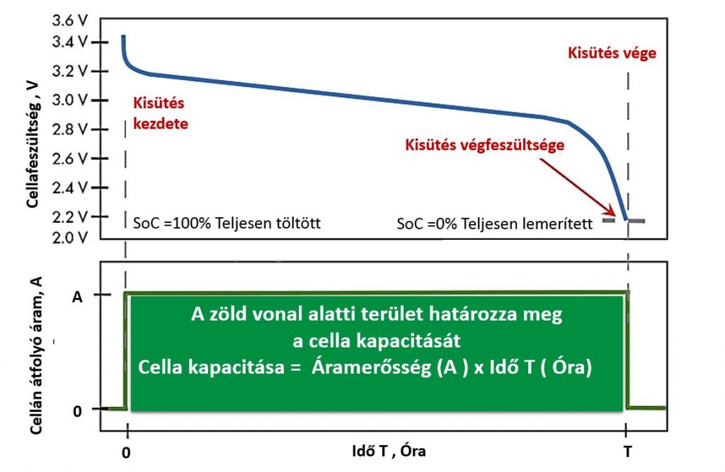
The voltage–time area alone is not capacity. The area under voltage against charge represents energy. Rated capacity refers to the manufacturer’s specified current, temperature and other test conditions. Constant current makes the calculation straightforward, but integrating measured current also permits non-constant-current charge accounting.
SoC expresses available charge relative to a defined reference capacity. The voltage–SoC relationship depends on chemistry and condition and is not generally linear. Hysteresis, temperature, load-induced voltage drop and ageing prevent terminal voltage from being a universally accurate SoC gauge. On a specified usable-charge scale, the upper reference state is assigned 100% and the lower reference state 0%; the reference capacity and endpoints must be stated. A cell’s nominal voltage remains a representative rating even while its actual voltage changes.
Energy: W = ∫U(t)I(t)dt = ∫U dQ, in Wh. Voltage multiplied by capacity requires constant or appropriately averaged voltage. Power: P = UI, in watts.
SoH describes condition relative to an initial or reference state. It may be defined through capacity, resistance or application performance. Report the definition and protocol: values calculated with different criteria are not automatically comparable. The original odometer analogy conveys accumulated history, but does not itself quantify remaining performance.
Why lithium-ion cells age
Cycling and storage can both cause capacity loss. A threshold such as 80% of initial capacity is a chosen test endpoint, not a universal boundary at which a cell becomes unusable or necessarily begins rapid failure.
Capacity loss may shorten operating time. Charging requires appropriate control and cell-specific voltage, current and temperature limits; habitual charging duration is not a substitute for a protocol.
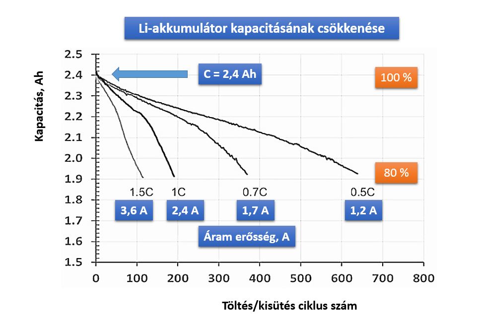
Current, temperature and upper voltage can influence ageing. Useful categories include loss of cyclable lithium, loss of active material and increasing resistance; the mechanisms and their relative importance depend on the cell and conditions.
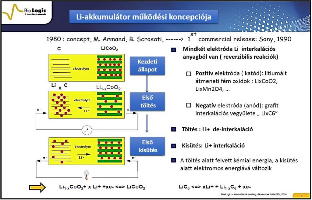
Initial cycles may consume cyclable lithium through irreversible processes such as interphase formation. This does not mean every cell necessarily retains metallic lithium after its first discharge. Later cycles may be more reversible, but side reactions can persist.
Possible processes include surface-film formation on either electrode, electrolyte oxidation or reduction, electrode passivation, metallic-lithium deposition, gas generation and reactions associated with structural changes in positive-electrode material. Water contamination can participate in unwanted chemistry, but it is not the only possible source of gas. None should be assumed solely from reduced efficiency. Testing provides evidence for investigation and cell selection rather than automatic identification of every mechanism.
Basic tests and their limits
Voltage, current, time and temperature provide a foundation. Capacity, cycle count and coulombic efficiency can be calculated from suitable data.
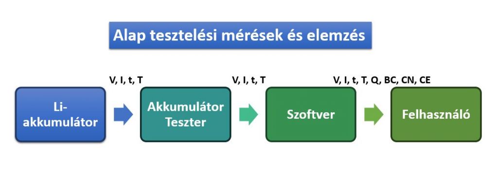
These measurements already contain useful information. Their limitations depend on the system: accuracy may be insufficient for a particular question, manual processing can burden long runs, software may lack required functions, and an oversimplified model may misrepresent the cell. Assess each limitation against the intended experiment rather than assuming every simpler tester is inadequate.
Potentiostats and galvanostats
Battery cells contain electrodes and electrolyte, so electrochemical instrumentation is useful in their study. A potentiostat controls potential and records current; galvanostatic operation controls current and measures potential. A reference electrode enables examination of an individual electrode potential. See how a potentiostat works.
Multiple independent channels enable parallel tests. The original illustration shows the historical VMP-3 platform.
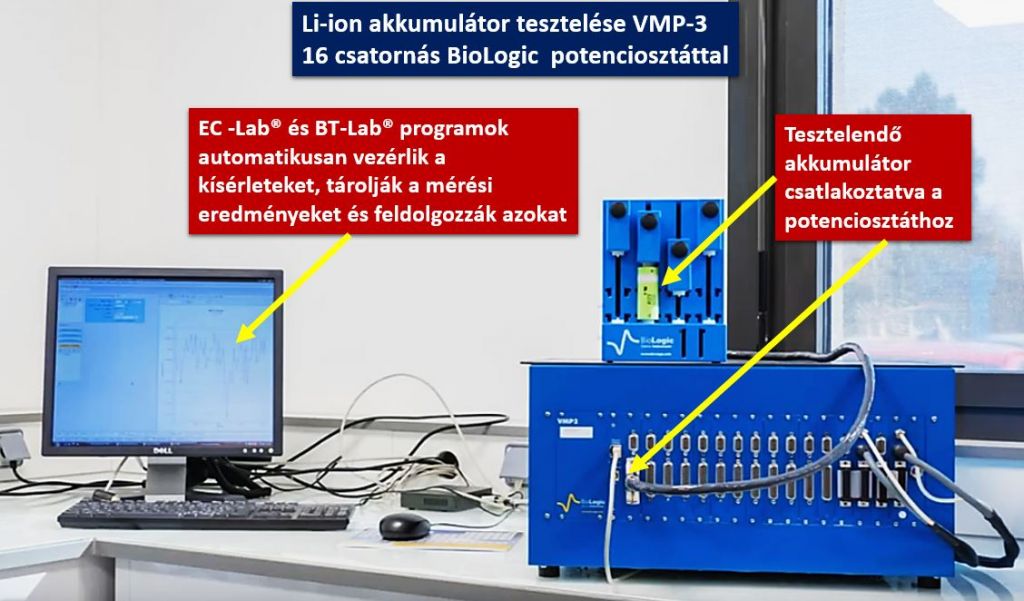
Pulse and EIS availability depends on the instrument, installed options and software. EIS is not a standard feature of every battery tester.
Connecting the cell
Four-terminal Kelvin wiring separates current-carrying and voltage-sensing leads, reducing the contribution of lead voltage drops to the measured cell voltage. It does not mean four independent measurement channels.
A two-terminal battery with four measurement leads still has two electrochemical electrodes. Do not confuse lead count with electrode count.
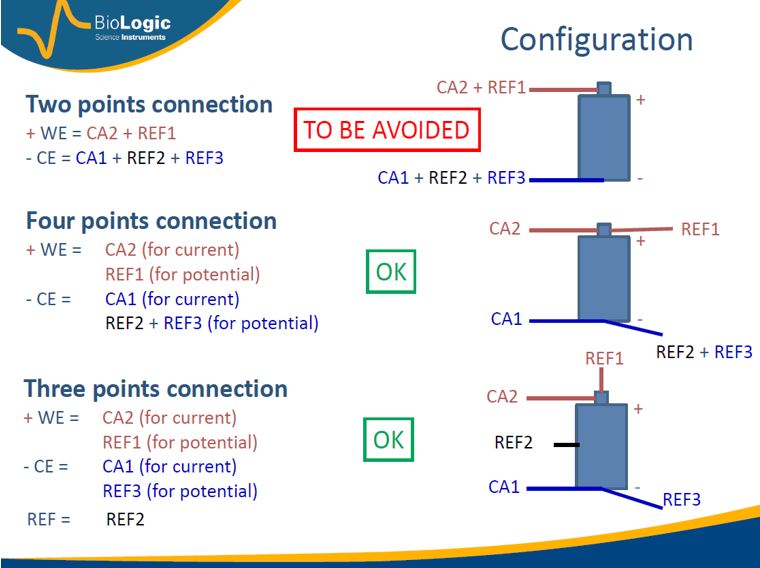
A separate reference is needed when individual electrode potentials must be followed. Follow the actual instrument manual and grounding requirements. Select a supported technique and set the limits before running it; preset software methods do not remove the need for a valid protocol.
BCD: battery capacity determination
The following methods retain the historical BCS-815/BT-Lab workflow. BCD determines capacity and can make the measured value available for later C-rate settings in techniques such as GCPL or ModuloBat.
A constant-current step moves the cell between selected voltage limits. Where the protocol requires it, a constant-voltage hold may follow until a specified current or time criterion is met.
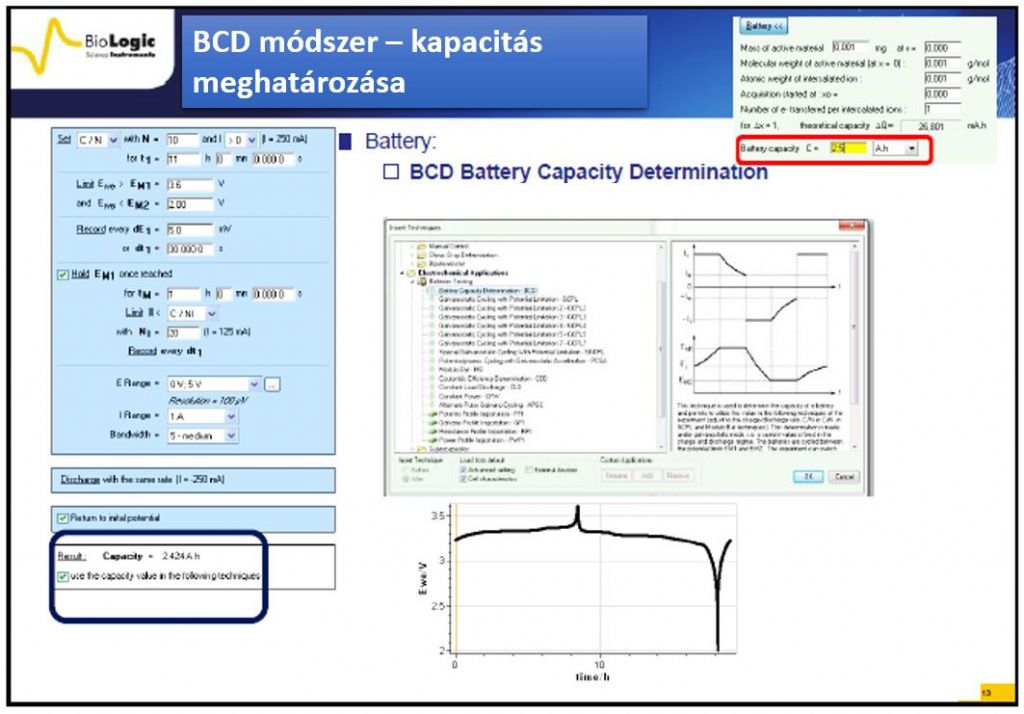
The historical BCD setup uses two voltage limits, labelled EM1 and EM2. Parameters and termination conditions are entered in the corresponding software fields. During a voltage hold, the current criterion Im and any time limit have different units and must not be confused. The Capacity result appears in the processing/output area. A subsequent charge or discharge can return the cell to a specified state, subject to its protocol. Capacity provides a useful baseline for later comparison.
The original workflow discusses CC (constant current), CV (constant voltage), CR (constant resistance), CP (constant power), VS (voltage scan), CI (current interrupt), PEIS (potentiostatic EIS) and GEIS (galvanostatic EIS). Availability and operating limits must be verified for the actual configuration; these modes do not all constitute the same capacity test.
CED and high-precision coulometry
Coulombic efficiency is CE = Qdis/Qch × 100% for consistently paired discharge and charge steps. Repeated cycles can include constant-voltage periods when required by the selected protocol.
High-precision coulometry (HPC) investigates small efficiency differences. The retained short-term and longer-term figures compare three original example cells measured with the historical BCS-815 setup. The early plot covers about 20 cycles; the longer comparison extends over approximately 100–350 cycles. These are the original study’s windows, not standard durations for all HPC experiments.
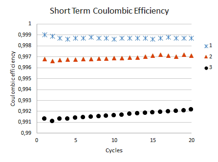
Differences close to unity require measurement uncertainty and stability appropriate to their size. Displayed decimal places are not proof of accuracy. Instrument performance, cell behaviour and temperature control all matter.
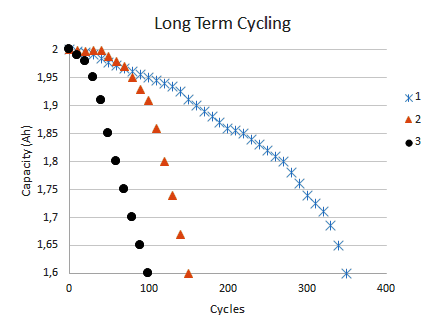
The figures illustrate a relationship between short-term efficiency and longer-term cycling in that experiment. They do not establish a universal lifetime guarantee. Side reactions can contribute to inefficiency, but high CE alone does not exclude every degradation mechanism.

Obtaining early evidence can reduce the time needed for comparing candidates, while long-term validation remains necessary. See BioLogic AN53 and the manufacturer HPC background.
GCPL and intermittent titration
GCPL means galvanostatic cycling with potential limitation. It applies constant-current charge/discharge with voltage limits. Current interruptions or planned rests add information about relaxation.
GITT alternates current pulses and rests. At constant current, ΔQ = IΔt. Voltage response and relaxation can support diffusion analysis under appropriate assumptions; the diffusion coefficient is not obtained simply from the current–time trace.
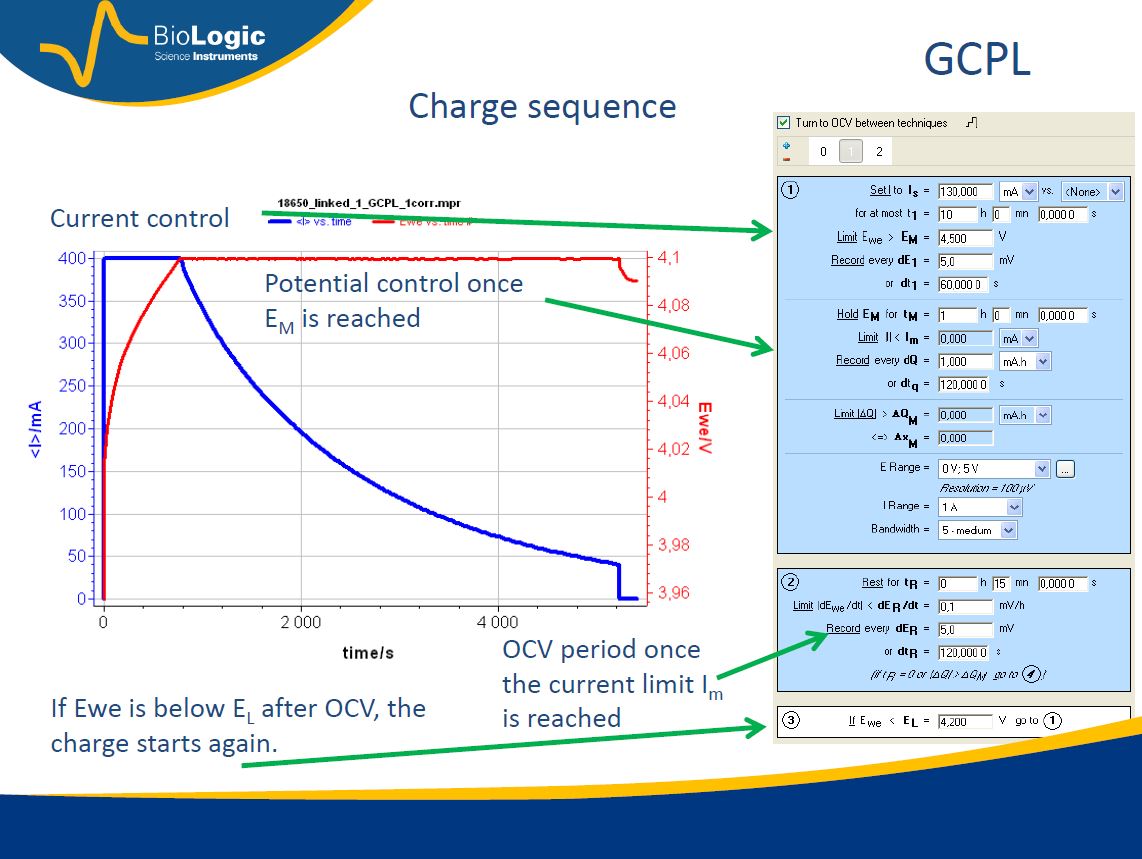
The retained curves show voltage changes during interruptions within a charge or discharge cycle.
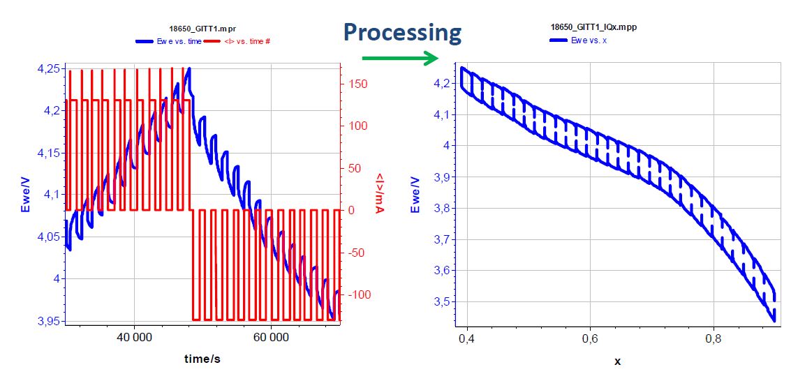
Charge can be related to composition: for one electron per ion and charge arising only from the reaction of interest, Δn = ΔQ/F. A stoichiometric coefficient x is dimensionless and additionally requires normalisation by the amount of active material.
The left side of the original GCPL plot shows the time trace, including the voltage excursions associated with interruptions; the processed representation relates voltage to composition on the right. The current and elapsed time determine transferred charge. Faraday’s constant converts charge in coulombs to electron equivalents, and the active-material amount is needed to convert those into composition. Potential–composition features may warrant investigation but do not prove an optimum lifetime. The original x = 0.7 observation does not establish a general discharge limit. Different GCPL variants and timing settings answer different questions; consult the method documentation and our GITT/PITT guide.
PCGA: potential-step characterisation
PCGA applies successive potential steps, whose duration can depend on current and time criteria. It is not simply a continuous linear voltage sweep. Integration of the transient gives ΔQ = ∫I(t)dt. BioLogic AN2.
Successive increments map charge against potential and, with the necessary normalisation, composition against potential. The retained LiCoO₂ example used +5 mV steps: its blue curve shows composition versus voltage, and the red curve the differential response.
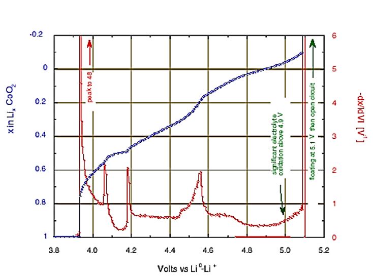
Peaks may be associated with phase transitions. Accompanying volume changes can cause mechanical stress and contact loss, but their magnitude is material- and state-dependent.
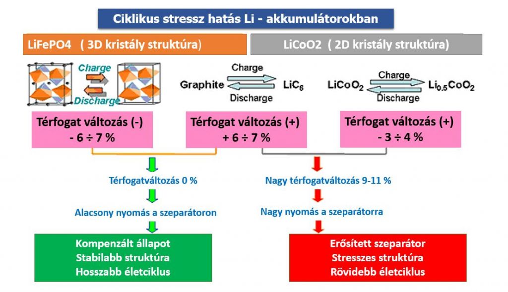
A single cycle can contain informative features, but their mechanism requires supporting evidence. Transient current provides kinetic information; diffusion or other contributions must be distinguished using the relevant assumptions. Potential-step characterisation and longer-term galvanostatic cycling are complementary rather than mutually exclusive.
DCA: differential capacity
DCA processes charge/discharge data to obtain dQ/dE, charge change per voltage change. Plateaus may appear as peaks and can help reveal structural changes.
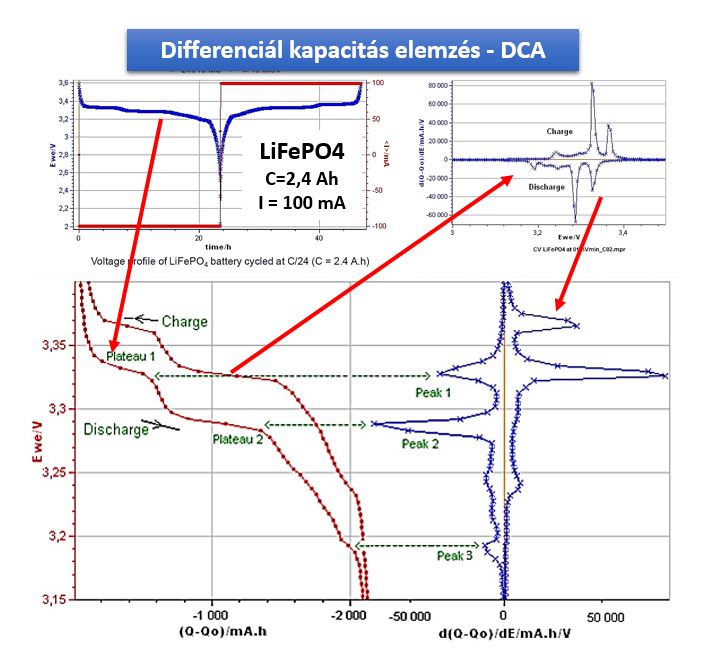
Loss of cyclable lithium and surface-layer formation may alter peak characteristics. However, peak changes do not uniquely establish lithium loss, plating or interphase growth; full-cell contributions and processing also matter. SEI denotes the solid-electrolyte interphase, not the whole electrolyte. See the DCA guide for sign conventions, sampling and smoothing.
Application or urban profiles
Real loads can differ substantially from a constant-current discharge. Recording a representative current or power profile can support a repeatable laboratory protocol, provided the tester can reproduce the relevant amplitudes and timing. The original workflow imports the recorded profile into the control software and runs the cell against it while recording capacity and other outputs. Recording terminal voltage alone does not necessarily define the load demanded by the application; specify what is controlled and what is observed. The control variable and termination conditions must be defined.
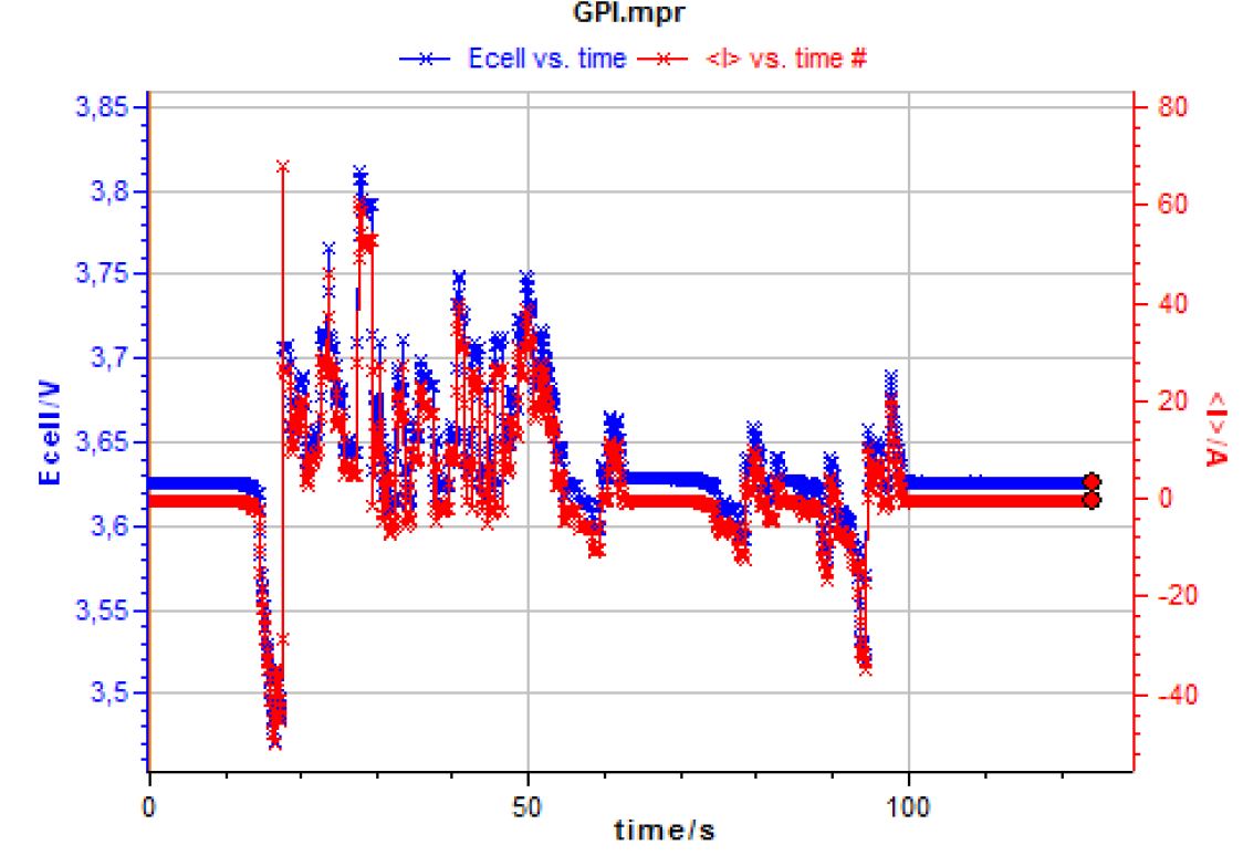
The original example compares a 40 Ah cell at 4 A with six repeated urban-profile segments. The temperature response is also shown. In that illustration the constant-current trace is green, the profile trace blue and the temperature trace red. The repeated profile produces temperature changes different from those during constant-current operation.
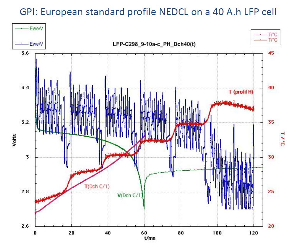
The illustrated temperature history differs between the profiles; it is an experimental observation, not a universal linear or stepwise rule.
EIS during cycling studies
EIS superimposes a small perturbation on a DC operating point and examines the response over frequency. Interfaces, electrolyte, contacts and slower transport may contribute on different timescales, often with overlap.
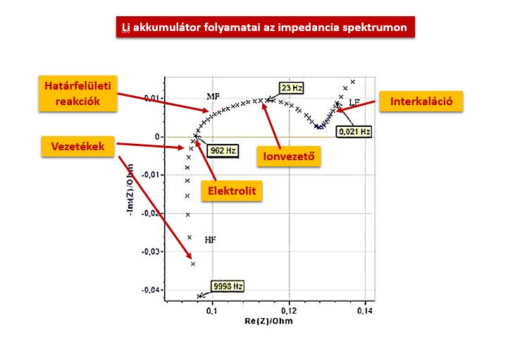
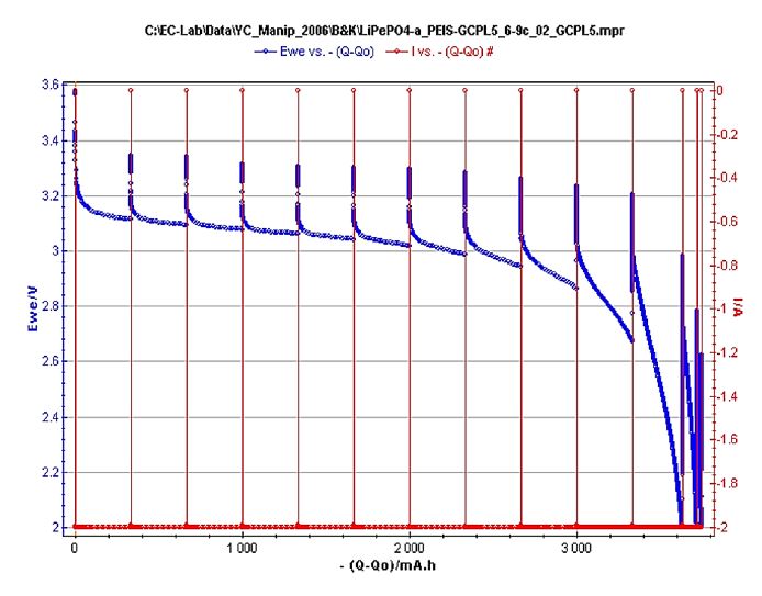
The retained protocol interrupts cycling to record spectra at selected states. Other DC operating points are possible when the measurement remains valid; rest duration and stationarity must be considered.
Compare spectra alongside SoC, temperature and ageing history. Our battery-test workstation article develops this example.
Equivalent circuits and state estimates
Fitting estimates parameters for a selected model. A close fit does not automatically prove uniqueness or physical assignments. The following BT-Lab screen is historical.
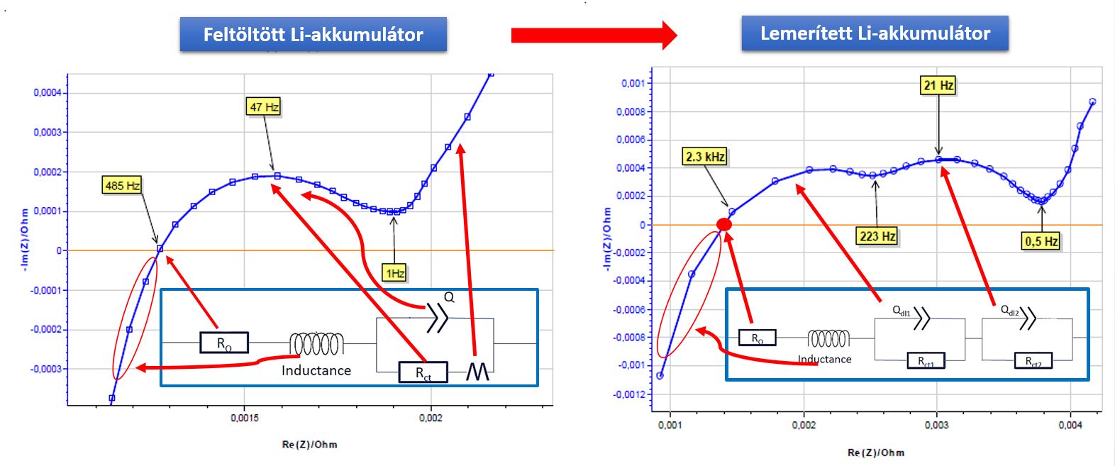
The next plot compares two states of charge, followed by the original fitted-parameter table. Quantitative comparison should retain the parameter definitions, units and fitting conditions. A reported “internal resistance” may describe one selected circuit element rather than every contribution to the cell response.
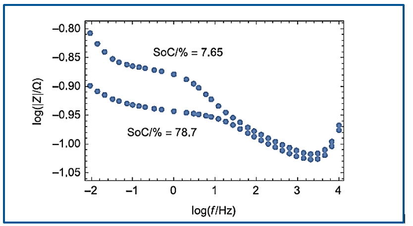
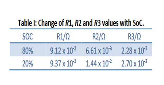
A relationship such as |Z| = f(SoC) may support estimation only after calibration and validation for the chemistry and conditions. Temperature, ageing and prior history also affect impedance. One discharge cannot establish a generally applicable conversion, and measurement duration depends on the frequency range and protocol.
Battery-module analysis
Appropriately configured channels can compare individual cells and a complete group. Channel isolation, common-mode limits and connection topology must support the arrangement.
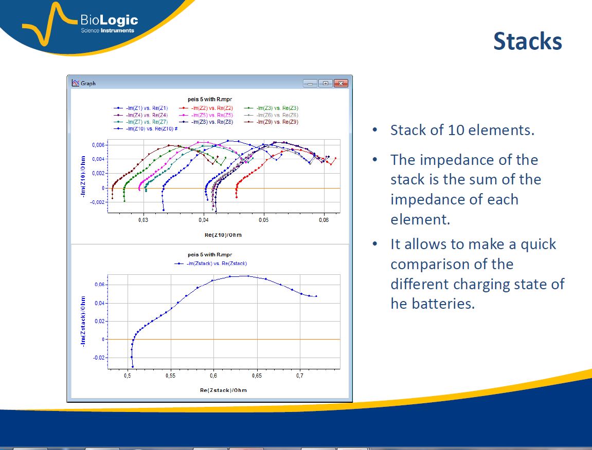
The retained example presents ten separate cell spectra and a combined response. Such measurements can investigate cell differences and module limitations; extracting SoC still needs a validated relationship.
Applying the methods
Capacity testing, HPC, intermittent titration, differential capacity, profiles and EIS provide complementary evidence. Choose methods for the research question, establish data quality and report limitations. Contact the Hungarian representative for help aligning the protocol and instrument configuration.