An EC Labor measurement guide with manufacturer references and our own calculated example.
Which question are you answering?
Before designing a titration experiment, separate the objectives: obtaining a near-equilibrium voltage curve, comparing transient shapes, or calculating a diffusion coefficient. The last requires additional assumptions. This guide uses an original calculation and a practical measurement plan to make those assumptions explicit.
GITT alternates current pulses with zero-current rests while recording voltage. PITT records the current transient following a potential step; integration gives the charge increment. A step can end on a time or current criterion. Not every protocol inserts an open-circuit interval between potential steps, so document the stopping condition alongside the technique name. BioLogic AN2: PITT protocols.
How much charge does one pulse transfer?
Original planning example: 1 mA for 600 seconds transfers 0.6 C, or 0.167 mAh. For an electrode previously measured to have 10 mAh capacity, that represents 1.67%. This calculation alone does not establish that the perturbation is sufficiently small at the composition being tested.
One hundred such pulses, each followed by a 3600 s rest, require 116.7 hours, almost five days. That excludes conditioning, repeats and interruptions. Selecting the rest time therefore also determines laboratory throughput.
Our suggested pilot experiment compares at least two pulse durations and two rest durations within the same state range. Define an acceptable residual voltage drift and the time window over which it is evaluated before the run. “One hour has elapsed” is a different condition from “the signal has stabilised.”
A conditional GITT equation
For the short-time planar diffusion approximation:
D = 4Lₑff²/(πτ) · (ΔEₛ/ΔEₜ)², with Lₑff = mVₘ/(MA).
Here τ is pulse duration, m active mass, Vₘ molar volume, M molar mass and A the modelled interface area. ΔEₛ separates relaxed voltages; ΔEₜ is the pulse voltage change excluding the ohmic jump. This requires a small perturbation, negligible kinetic contribution and τ ≪ L²/D; the analysed transient must also follow square-root time dependence. It is not a universal particle model. BioLogic AN70: diffusion analysis.
Worked example and geometry sensitivity
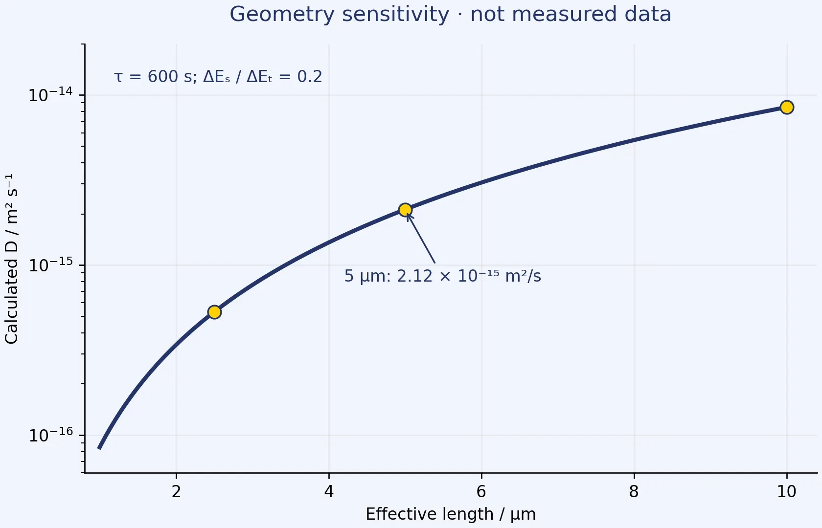
Choose teaching values of Lₑff = 5 µm, τ = 600 s, ΔEₛ = 2 mV and ΔEₜ = 10 mV. The equation gives D ≈ 2.12 × 10⁻¹⁵ m²/s, equivalent to 2.12 × 10⁻¹¹ cm²/s. This is a calculated example, not a measured property of a particular material.
If L = Lₑff in this planar example, L²/D is approximately 11,781 s: the pulse occupies about 5.1% of that interval. This is a useful ratio check, but it does not independently validate the model.
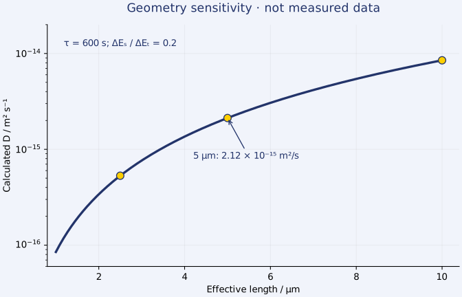
Keeping the voltage values unchanged, a length of 2.5 µm gives one quarter of the calculated D; 10 µm gives four times D. Even this simple equation is strongly affected by geometry assumptions. The figure illustrates that sensitivity, not differences between materials. Download the original calculated figure as SVG.

What makes the interpretation defensible?
Particle-size distribution and the transport model affect parameters extracted from GITT. Horner and colleagues modelled the full pulse and relaxation, then checked results against independent cycling predictions. A good fit is therefore one check; predicting a separate experiment can provide another. Original research on GITT modelling.
Suggested measurement record
- Record the sample, temperature, conditioning, state of charge and electrode roles.
- Specify the pulse, rest, sampling and every stopping condition.
- Save the beginning of the raw transient and identify the interval selected for analysis.
- Distinguish measured geometry from the area or length assumed in the model.
- For PITT, retain current–time data alongside integrated charge; for GITT, retain the complete relaxation.
- Report excluded points, units and sensitivity calculations.
Start instrument selection with concrete requirements: pulse current, low-current measurement needs, voltage window, reference electrode and parallel channels. The instrument finder provides a shortlist; suitability of the MPG-200 family or another system requires confirmation of the exact configuration. For a complementary frequency-domain method, read the EIS guide.