Introduction
Differential capacity analysis (DCA), also called incremental capacity analysis (ICA), supports the study of rechargeable-battery ageing by following peaks associated with changes in active materials. Lithium-ion degradation is complex. Loss of conductivity, loss of active material and loss of lithium inventory are useful categories, but a peak change alone does not uniquely identify a mechanism. A full-cell response combines contributions from both electrodes.
The usual representation is dQ/dE against E, also written dQ/dV against V. Plateaus in a voltage–charge curve become peaks in differential capacity. Peak position, height, width and area can be followed between cycles. Charge and discharge profiles also provide evidence relevant to reversibility. Original manufacturer background.
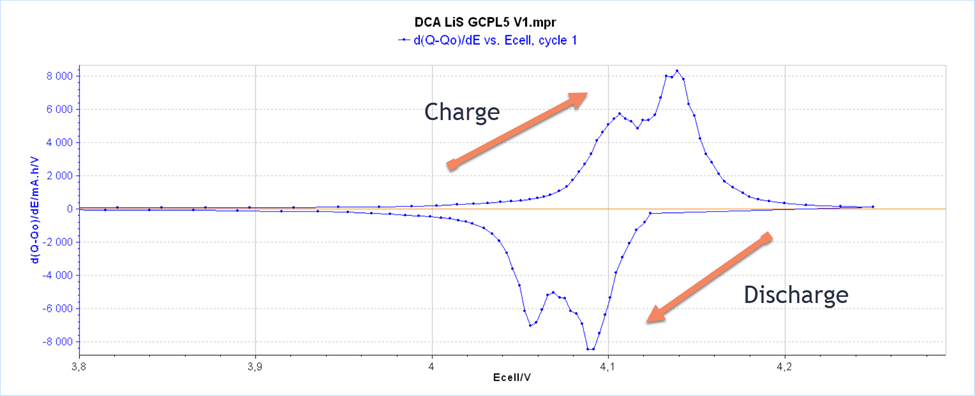
Figure 1. Typical differential-capacity representation, retained from the original article.
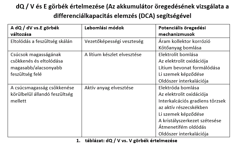
Side reactions may involve electrolyte, active material, current collectors or binders. The retained table summarises possible relationships between degradation modes and peak characteristics; it is not a standalone diagnostic rule.
Differential and incremental capacity processing
The original article describes EC-Lab DCA processing using constant voltage-increment recording, and DCS processing for constant-time recording. Its Advanced Option selects the voltage increment used for differentiation. The exact interface depends on software version.
Locally retained BioLogic AN40 PDF provides the historical example below. DCA/ICA has been available since EC-Lab 10.21, released in May 2012. The example uses slow cycling; its settings are not universal requirements.
Differential capacity is obtained from the charge–voltage curve. The historical equation uses the absolute charge increment divided by the signed voltage increment:
|dQ|/dE ≈ |Q₂ − Q₁|/(E₂ − E₁).
Q₂ and E₂ refer to a recorded point; Q₁ and E₁ to the preceding point. Under this convention, decreasing voltage produces a negative discharge branch.

The retained manufacturer experiment
The AN40 example tested commercial 2.5 Ah LiFePO₄ cells at room temperature between 3.6 V and 2.0 V, using C/25 constant current. The instrument was an MPG2 battery cycler controlled by EC-Lab 10.21. These are historical experiment conditions, not charging instructions for an arbitrary cell.
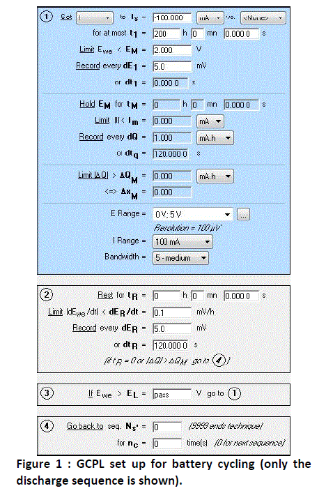
The procedure first charged the cell fully to 3.6 V, discharged at C/25 to 2.0 V, then charged at C/25 to 3.6 V. During the discharge and charge steps, points were recorded at each selected voltage increment dE₁; the time-recording parameter dt₁ was disabled by setting it to zero.
Results from the original example
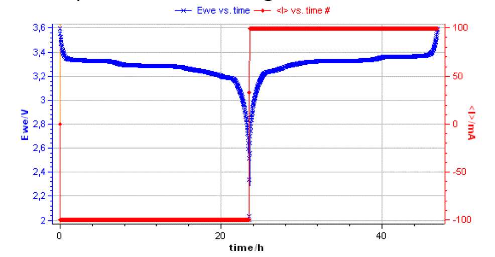
Figure 2. Retained discharge and charge voltage trace.
In the EC-Lab 10.21 Process Data window, the original example selected d(Q−Q₀)/dE, charge capacity and discharge capacity. These historical screenshots document that workflow.
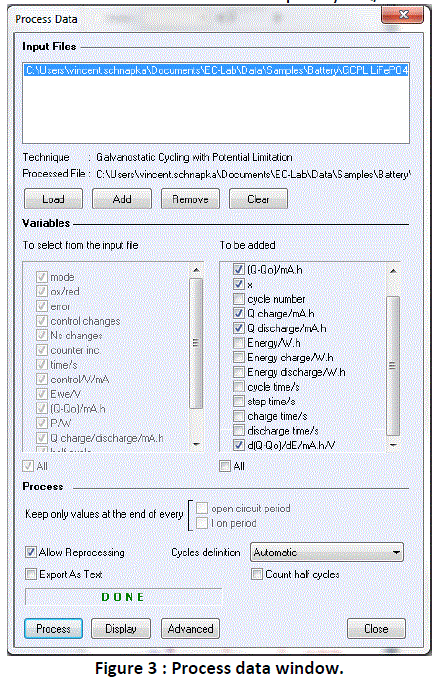
The processed curve can be displayed against voltage, charge or another parameter. The two retained plots present differential capacity against voltage and the same information with reversed axes.
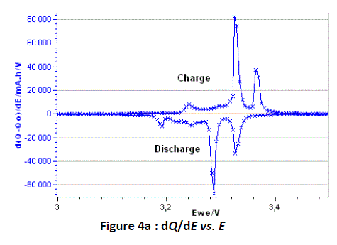
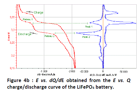
The original example identifies four main peaks: two during discharge and two during charge. They correspond to plateaus in the voltage–charge profile, interpreted in the example as two-phase coexistence. This interpretation must remain tied to the particular cell and experiment.
DCA makes features in cycling data easier to compare and can support investigation of intercalation-material changes. It does not independently establish a unique degradation mechanism or its kinetics. The original article also links to a DCS example in BioLogic AN57.
An original numerical example
For a general finite difference, dQ/dV ≈ (Q₂ − Q₁)/(V₂ − V₁), in units such as Ah/V. Always specify whether the numerator is signed or absolute before comparing curves.
Our invented charge data are Q₁ = 1.000 Ah, Q₂ = 1.012 Ah, V₁ = 3.400 V and V₂ = 3.402 V. The ratio is 0.012 Ah / 0.002 V = 6 Ah/V. This is an average slope over a finite interval, not an exact point derivative. At a constant 0.100 A, that 0.012 Ah increment takes 0.12 hours, or 432 seconds.
If the recorded voltage difference were 1 mV instead of 2 mV, the same numerator would give 12 Ah/V; at 3 mV it would give 4 Ah/V. This sensitivity example is not an uncertainty estimate. It shows how a small denominator amplifies voltage differences. At zero ΔV, the ratio is undefined; do not replace it with an arbitrary finite peak.
Sampling, noise and smoothing
Sampling and smoothing can change the resulting peaks. Smoothing Q(V) before differentiation and smoothing the resulting dQ/dV curve are different operations. Lower cycling rates can reduce kinetic contributions without making mechanism identification automatic. Dubarry and Anseán: methodological study.
Our suggested check processes the same raw dataset with two justified voltage increments and two modest smoothing settings. Record which peaks persist and changes in position, height or area. This tests sensitivity rather than selecting the most attractive curve.
Treat charge and discharge separately. Do not merge rest periods, current changes or constant-voltage steps into one monotonic charging branch without checking them. Differences between cycles cannot simply be assigned to ageing if temperature, protocol and processing differ.
What should be retained for interpretation?
- Raw time, current, voltage and charge data, cell identifier and cycle number.
- Differentiation method, voltage increment, smoothing window and sign convention.
- Excluded sections and integration boundaries for peak areas.
- The proposed mechanism and separate evidence supporting it.
The battery-cycler guide adds worked charge and energy examples. Internal-resistance measurement supplies a complementary view; neither method automatically replaces the other.