
Corrosion measurements support the development of protection strategies. Investigations can be labour- and time-intensive. Under suitable conditions, electrochemical methods can provide a relatively quick estimate of uniform corrosion rate; stabilisation and long-term validation remain necessary.
Corrosion usually degrades material properties. Measuring its rate and investigating mechanisms can help identify suitable protection measures.
Metal corrosion in aqueous environments couples anodic dissolution to a cathodic reaction. Measuring current and potential while changing solution conditions can provide useful information. At open circuit, external net current can be zero while metal still corrodes: Icorr represents the magnitude of the balancing partial currents. BioLogic potentiostats and EC-Lab support these measurements and their analysis.
Performing corrosion measurements
Corrosion is commonly described as uniform or localised. With uniform corrosion, material loss is distributed relatively evenly across the surface, so an average penetration-rate estimate may be useful. For localised attack, that average does not describe the deepest damage.
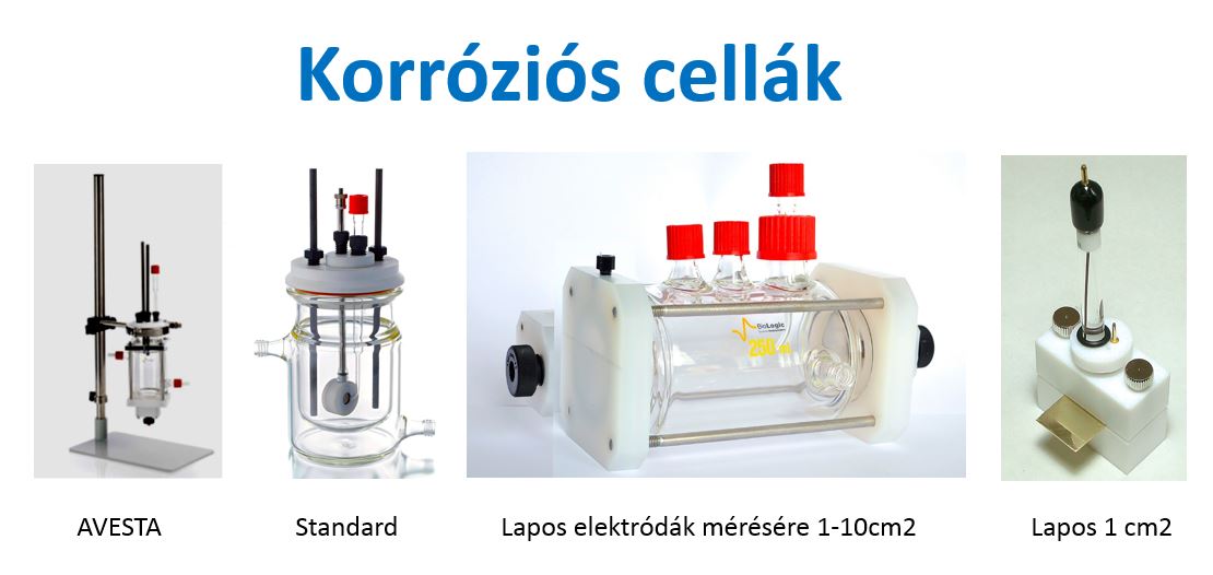
Electrochemical investigation requires a suitable potentiostat and corrosion cell.
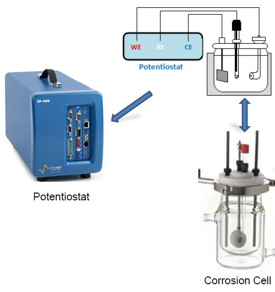
The SP-150 in the original article is a historical example. For current configuration planning, see the SP-150e and instrument finder. Check current range, cell voltage and EIS options separately. Contact info@labornite.hu to discuss the instrument and cell for your experiment.
The overall electrochemical reaction combines two half-reactions:
- Oxidation, electron loss: Red → Ox + ne⁻.
- Reduction, electron gain: Ox + ne⁻ → Red.
Oxidation increases oxidation state; reduction decreases it. Oxidation state is formal electron bookkeeping, not generally the actual atomic charge. For a monatomic ion it equals the charge number. Examples include zero for elements such as Fe, Ni, O₂ and H₂; positive values for Fe²⁺, H⁺, Na⁺, Cu²⁺ and Al³⁺; negative values for Cl⁻ and O²⁻.
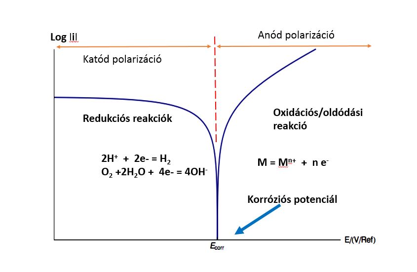
The graph illustrates the corrosion potential and partial reactions. Ecorr can be considered alongside equilibrium redox potentials, but its time evolution alone does not establish corrosion rate or passivation. Interpret it with current, resistance and surface information.
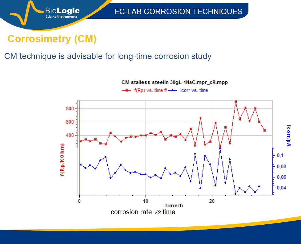
Software supports calculation and analysis; the user must still check the model and fitting interval. Under Stern–Geary conditions and with the same B coefficient, Icorr = B/Rp. A larger Rp then implies a smaller corrosion current. B can change between media and mechanisms, so Rp alone is not a universal corrosion-rate scale.
Example: iron in an acidic solution
The original article includes a BioLogic AN10 example comparing Tafel and Rp fitting. Its reported configuration is:
- Iron rotating-disc working electrode, area 0.0314 cm², rotation 800 rpm.
- Platinum-wire counter electrode.
- Saturated calomel reference electrode, SCE.
- 0.1 M HCl solution.
The potential scan spans −0.6 to 0 V versus SCE. The archived source contains a discrepancy: its prose gives 10 mV/s, while the settings list and screenshot show 50 mV/s. This is not a verified measurement recipe. The actual rate must be resolved from raw files; neither value is presented here as universally quasi-steady.
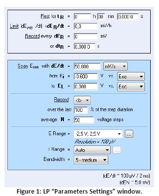
The prose specifies SCE, while the screenshot displays a different reference setting; this also requires checking against the raw file. The archived LP settings also show recording over the last 100% of each step, averaging 50 voltage steps, automatic current range and bandwidth 5, medium. The historical note associates a ±1 V control span with a potential-step resolution change from 300 to 50 µV. These are configuration-specific historical settings; consult the documentation for the actual instrument and software in use.
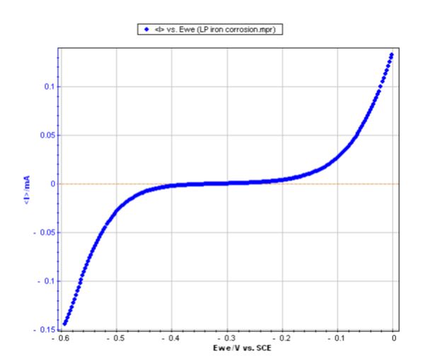
Stern method: Tafel fit
Using positive magnitudes for the anodic and cathodic Tafel slopes:
I = Icorr[exp(ln(10)(E − Ecorr)/βa) − exp(−ln(10)(E − Ecorr)/βc)].
The negative sign in the cathodic exponent matters. This corrected text replaces an old equation image with a missing sign.
Analysis of E and log|I| can estimate Icorr, Ecorr and the Tafel slopes when the assumed kinetic relationship is applicable. EC-Lab provides a Tafel fitting tool.
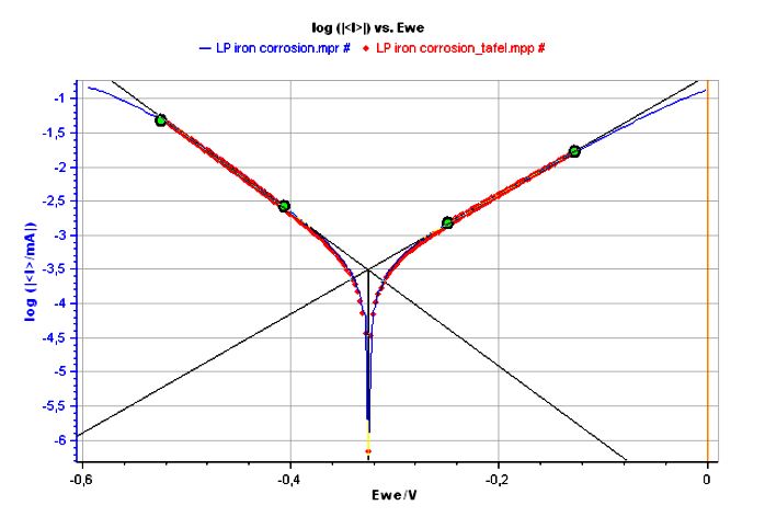
Converting corrosion current to a penetration rate also requires equivalent weight, material density and exposed area. For a pure metal dissolving with a known electron count, equivalent weight is molar mass divided by that count.
Stern–Geary method: Rp fit
Polarisation resistance is Rp = dE/dI at Ecorr, the reciprocal of dI/dE:

For the two-Tafel-branch relationship above:

Thus Icorr = βaβc/[Rp(βa + βc)ln(10)]. The EC-Lab Rp tool estimates the slope around the corrosion potential. Converting it to Icorr also requires suitable βa and βc values.
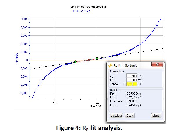
The historical example reports:
- Tafel fit: Icorr = 0.310 µA.
- Rp fit: Icorr = 0.416 µA.
Their difference is approximately 34% relative to the Tafel result. Without uncertainty estimates this is not demonstrated agreement. The example also reports a penetration-rate estimate of 0.116 mm/year; this is specific to that dataset and conversion assumptions.
Cyclic potentiodynamic polarisation
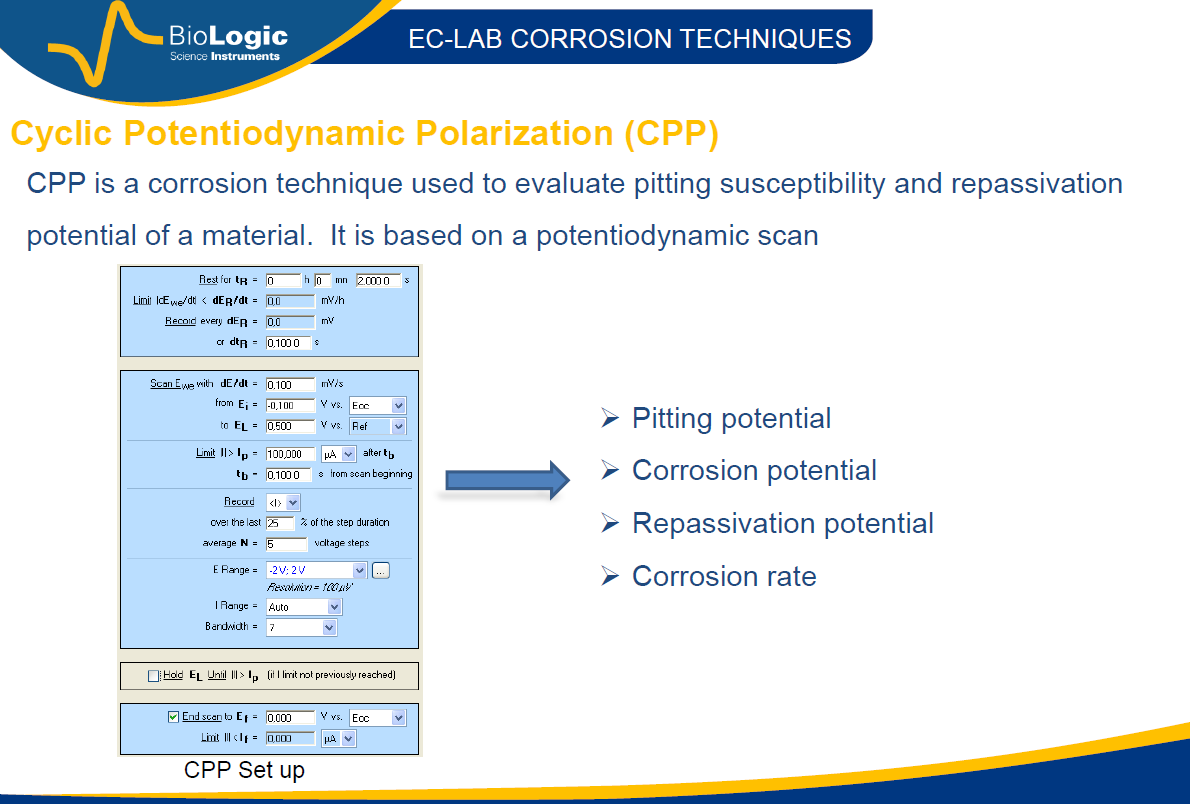
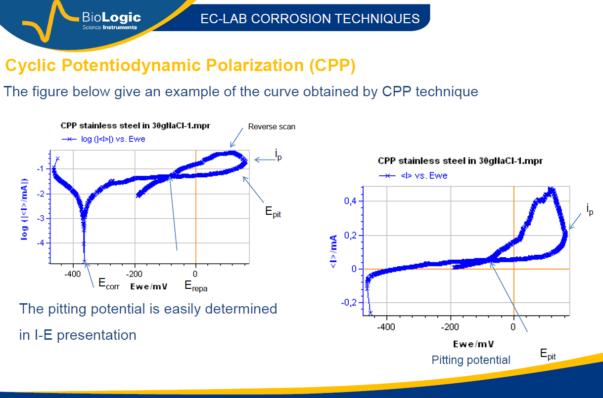
CPP can help characterise pitting and repassivation under defined test conditions. The associated potentials depend on the environment, surface and protocol; the hysteresis loop alone does not give a universal corrosion rate. A potentiostat can execute the programmed scan, while interpretation still requires a suitable experiment.
Parallel corrosion measurements
An appropriately configured multichannel BioLogic instrument can perform measurements on up to 16 independent channels. Parallel work can increase throughput; it does not guarantee a sixteenfold reduction in total research time. Sample preparation, cells, stabilisation and analysis can remain limiting factors.
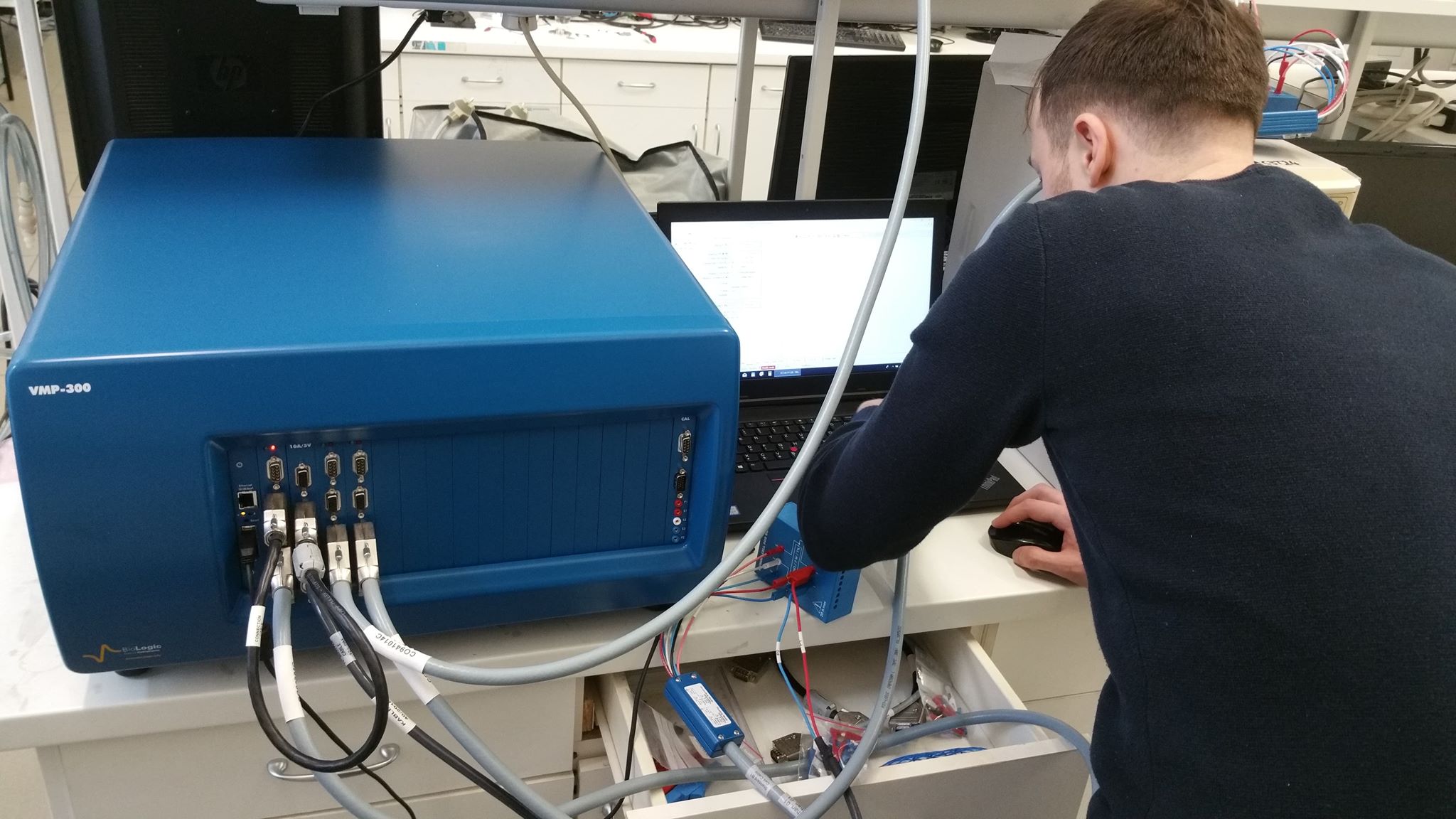
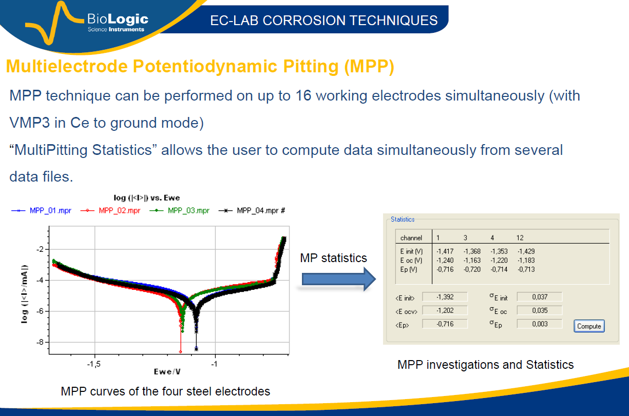
The retained example illustrates four steel electrodes measured in parallel on one multichannel potentiostat. Earlier results can support faster development when the complete workflow benefits.
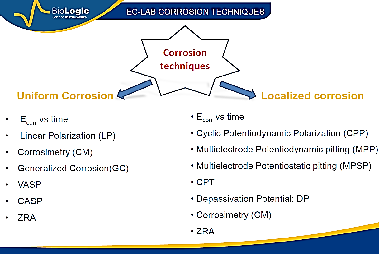
Corrosion methods available with BioLogic instruments
Characterising corrosion by EIS
Electrochemical impedance spectroscopy probes the response around an operating point using a small AC perturbation. Check linearity, stationarity and causality. A corrosion operating point is not necessarily thermodynamic equilibrium. Small excitation does not guarantee a fast or completely non-destructive experiment.
EIS can support separation of processes with different time scales. Circuit parameters become corrosion descriptors only through an appropriate physical model. VASP and CASP are specific corrosion techniques described in AN36 and AN37. A generic EIS spectrum does not automatically provide Icorr.
Treat solution resistance and mass transport separately. In a simple system without adsorption or diffusion limitation, an uncorrected DC slope can contain Rp + RΩ. EIS may separate them when the spectrum and model allow it. Error direction is not universal across methods. BioLogic AN48.
The original article presents a stainless-steel spectrum in 1 M HCl, with measured data in blue and fitted values in red:
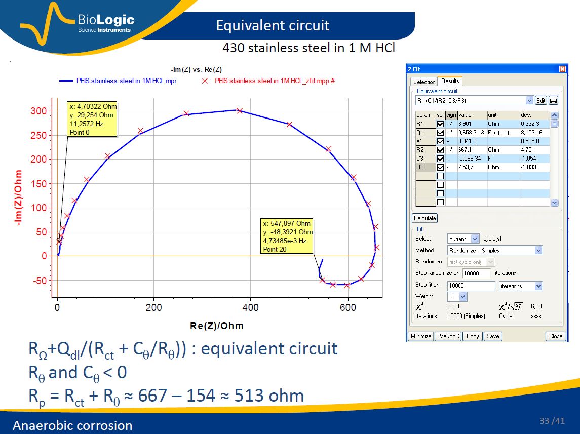
Fitting can test mechanistic hypotheses, but similar or identical spectra may admit different models. The following Faradaic-impedance model is retained from the original article:
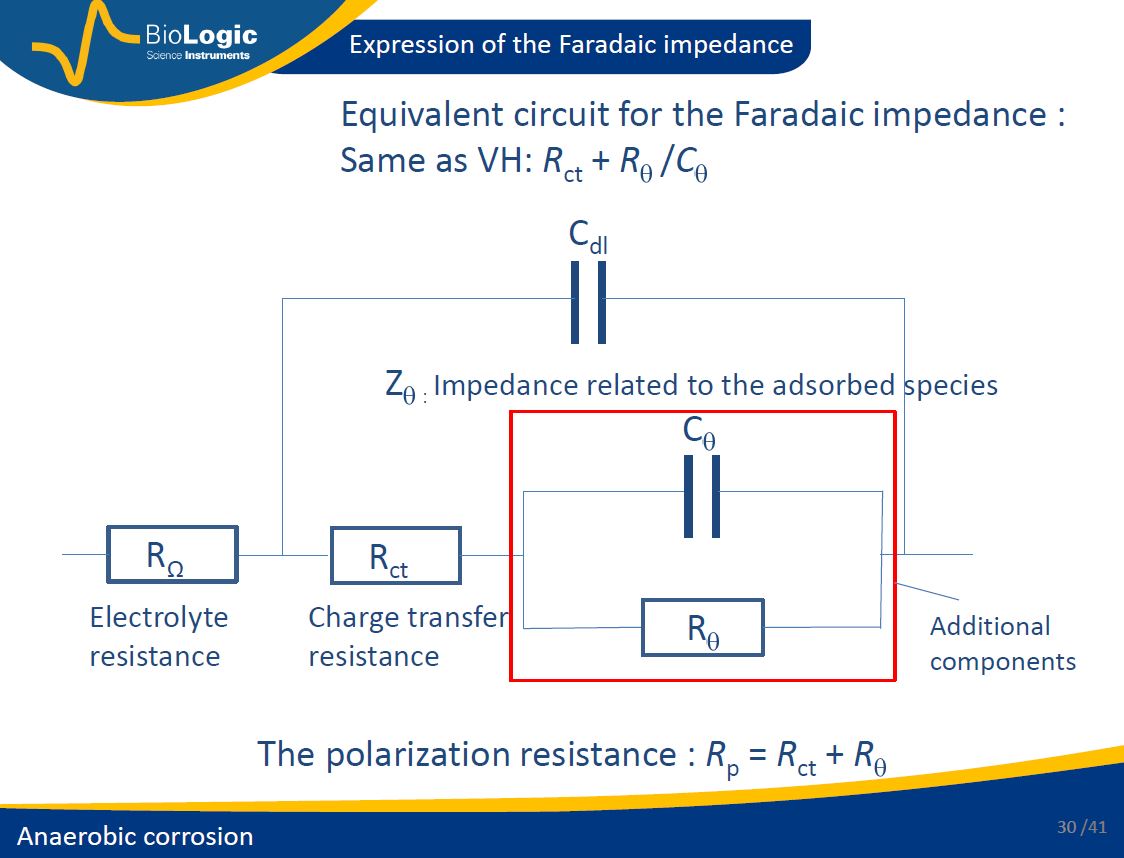
- In a simple Tafelian system, the model RΩ + (Cdl ∥ Rct) can describe charge-transfer-controlled behaviour and permit Stern–Geary analysis under its assumptions.
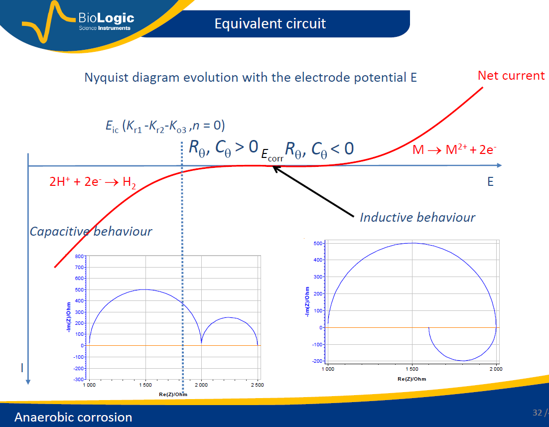
- With adsorption, as in a Volmer–Heyrovský-type mechanism, a low-frequency inductive loop can occur and Rp may differ from Rct. These resistances cannot automatically be substituted for each other; reassess the usual two-Tafel-branch analysis. Manufacturer model discussion.
BioLogic instruments and EC-Lab support corrosion measurement and analysis. Check functions against instrument configuration and software version. Multichannel work can increase throughput, while EIS duration depends on the lowest frequency, period count and settling. At 10 mHz one period lasts 100 s; three periods take five minutes before any other frequencies.
Choosing a method: editorial addition
- LPR: use a small perturbation around Ecorr to estimate the slope. Check linearity, settling and solution resistance. Without B, the result is Rp rather than an unambiguous corrosion rate.
- Tafel: establish a near-linear kinetic region in E–log|I|. Do not automatically fit a diffusion plateau, passivation region or rapidly changing surface as a Tafel branch.
- EIS: useful when separating ohmic, charge-transfer and additional contributions. Model validity and data quality determine what is identifiable.
Our original illustrative calculation, not a new measurement: take βa = βc = 0.120 V/decade and area-normalised Rp,A = 2000 Ω·cm². Then B = βaβc/[ln(10)(βa + βc)] ≈ 0.0261 V, so jcorr = B/Rp,A ≈ 13.0 µA/cm². For 2.0 cm², Icorr ≈ 26.1 µA. Rp in Ω gives current; Rp,A in Ω·cm² gives current density. Keep these quantities distinct.
Record the area definition, pretreatment, medium, temperature, reference, stabilisation criterion, fitting interval and repeats. State whether B was measured or assumed. Related guides: EIS data quality and EIS fitting.