An EC Labor measurement guide with manufacturer references and our own calculated example.
What does fitting provide?
An equivalent circuit describes impedance as a function of frequency and model parameters. Fitting estimates those parameters. Agreement between curves does not establish the proposed physical processes: different circuits can produce identical impedance. EC-Lab’s ZFit tool fits such circuits. BioLogic AN14: equivalent circuits and ZFit.
Begin by checking EIS data quality. Poor data can still yield an impressive-looking fit; numerical agreement does not replace checking measurement conditions.
Our example: a missing series resistor
Generate synthetic data from Rₛ + (R ∥ C) with Rₛ = 5 Ω, R = 80 Ω and C = 100 µF:
Z(f) = 5 + 80/(1 + j2πf·0.008) Ω.
Use 70 logarithmically spaced frequencies from 0.1 Hz to 10 kHz. Add independent, zero-mean Gaussian noise with a standard deviation of 0.2 Ω to the real and imaginary components, using a fixed random seed. This is a teaching dataset, not a measurement or claim about instrument accuracy.
Fit two models with identical unit weighting:
- Rₛ + (R ∥ C): Rₛ ≈ 5.001 Ω, R ≈ 80.022 Ω, C ≈ 99.963 µF.
- R ∥ C: R ≈ 84.497 Ω, C ≈ 88.346 µF.
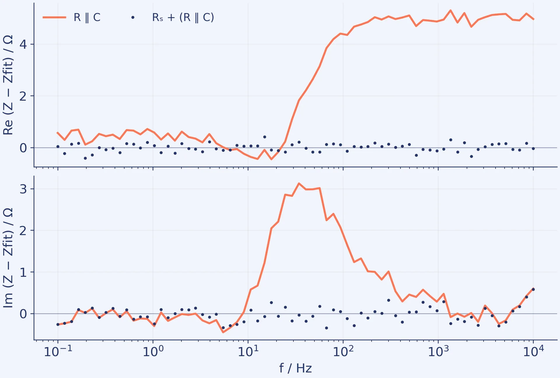
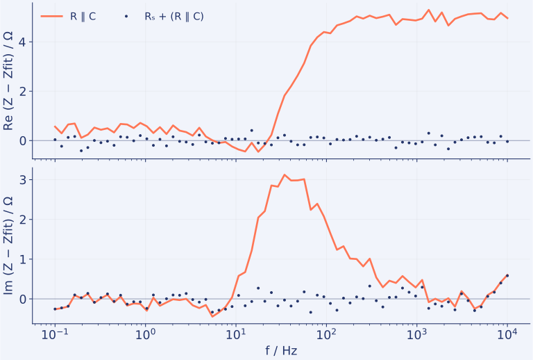
The second model omits the series resistor. The combined root-mean-square of the 140 real/imaginary residual values is 0.170 Ω for the first model and 2.480 Ω for the second. This statistic describes this particular dataset; it is not a universal acceptance threshold.
Plot the residuals too
Define ΔZ = Zdata − Zmodel. Plot real and imaginary residuals separately against frequency. Our figure shows structured deviations when the series resistor is omitted. The other model leaves smaller deviations on the scale of the added noise. Download the calculated figure.

Here we know what is missing because we generated the data. For experimental spectra, a similar pattern does not identify the cause by itself: examine the model, measurement settings and sample. Retain both raw and reconstructed Nyquist and Bode plots.
What does weighting change?
One possible objective is S = Σ wₖ[(Re ΔZₖ)² + (Im ΔZₖ)²]. Unit weights minimise absolute deviations. Our numerical example: a 0.1 Ω deviation is 10% of a 1 Ω impedance magnitude, but 0.1% of 100 Ω. Absolute and relative errors therefore assign different priorities to a fit.
Document any weighting based on measurement variance. Different real/imaginary uncertainties may require separate weights instead of the common weight above. Do not directly compare objective values obtained with different weighting or frequency lists. Record the software’s precise definition of χ² too.
How certain are the parameters?
ZFit’s “std err.” describes uncertainty associated with the estimated parameter. Manufacturer examples show effects from noise, model choice and incomplete frequency coverage. BioLogic: interpreting standard error.
A small error estimate does not establish a mechanism. As editorial checks, try multiple initial guesses, inspect parameters reaching their bounds and examine changes under reasonable fitting settings. Distinguish numerical stability from physical correctness.
When is the circuit too complex?
An additional parameter can improve agreement without being well determined. Frequency-dependent parameter sensitivity can help identify poorly justified elements. BioLogic: ZFit sensitivity factors.
An identifiability example: two series resistors enter the impedance only through R₁ + R₂. The same spectrum cannot distinguish a 3 + 2 Ω split from 4 + 1 Ω. More decimal places cannot resolve this. Our DRT guide gives a related time-constant counterexample.
Save the topology, initial guesses, bounds, weighting, frequency limits, residuals, uncertainties and software version with the result. Write down the physical justification separately. The EC-Lab and EIS basics pages connect measurement planning with analysis.