An EC Labor measurement guide with manufacturer references and our own calculated example.
What question does DRT answer?
The distribution of relaxation times (DRT) examines the time constants represented in an impedance spectrum. It can help select an equivalent circuit when Nyquist arcs overlap. This is another representation of existing EIS data, not a new measurement. The manufacturer’s overview discusses both its potential and limitations in separating peaks. BioLogic: DRT and equivalent circuits.
Start with our EIS introduction if impedance interpretation is new to you. Check data quality before calculating DRT: computation cannot repair a cell that changed during measurement.
Our example: two known RC elements
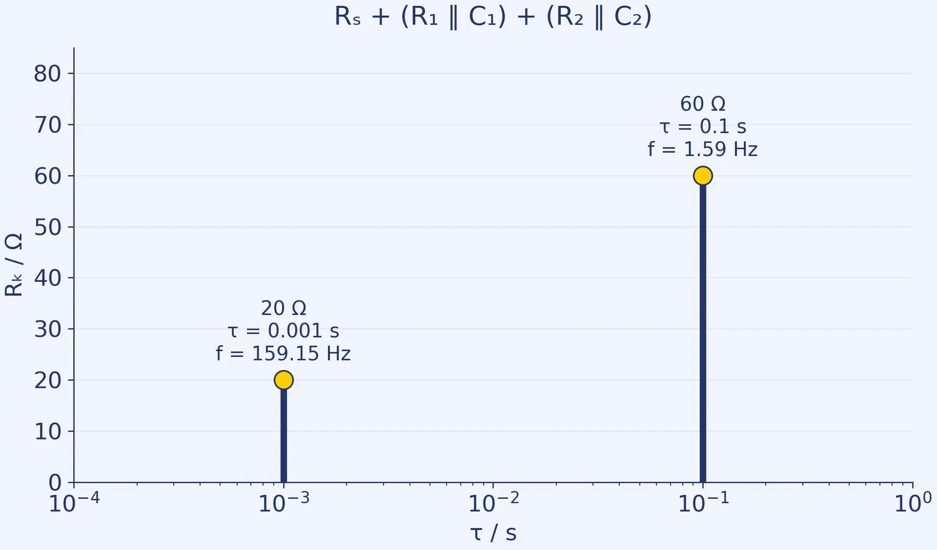
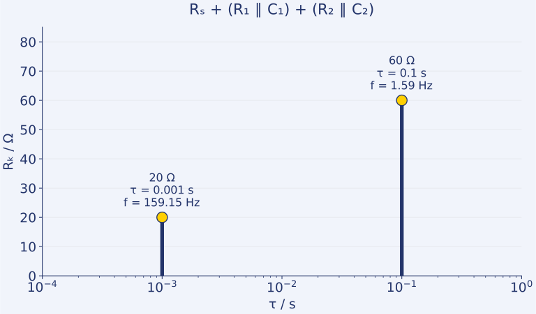
Consider the ideal circuit Rₛ + (R₁ ∥ C₁) + (R₂ ∥ C₂). Choose Rₛ = 5 Ω, R₁ = 20 Ω, C₁ = 50 µF, R₂ = 60 Ω and C₂ = 1.667 mF, the last value rounded. Then:
Z(ω) = 5 + 20/(1 + jω·0.001) + 60/(1 + jω·0.1) Ω, where ω = 2πf.
The time constants are τ₁ = 0.001 s and τ₂ = 0.1 s. Each RC element has a characteristic frequency fₖ = 1/(2πτₖ), giving 159.15 Hz and 1.59 Hz. These need not be visible peak positions in the combined spectrum.
At high frequency, total impedance approaches 5 Ω; at low frequency, 85 Ω. The two relaxations contribute 80 Ω in total. The series 5 Ω is separate.
Our figure shows known discrete resistance weights, not a DRT recovered from noisy data. Stem heights represent Rₖ, not a continuous distribution density. Download the vector figure.

Peak height or peak area?
One continuous representation is:
Z(ω) = Rₛ + ∫ γ(ln τ)/(1 + jωτ) d ln τ, integrated over the full logarithmic time-constant domain.
With this convention, γ has units of Ω and its integrated area gives the resistance contribution. An ideal RC element corresponds to a Dirac peak. Other definitions, such as density with respect to dτ, require different normalisation. Compare peaks only under the same convention. BioLogic AN60: theoretical background.
Why is regularisation necessary?
Recovering a distribution from finite, noisy data is an ill-conditioned inverse problem: small data changes can produce large distribution changes. Regularisation considers, for example, solution smoothness alongside data agreement. The chosen penalty therefore forms part of the modelling assumptions. Ciucci and Chen: regularisation and Bayesian DRT.
Too little smoothing can leave noise-related peaks; too much can merge separate contributions. Compare multiple settings, reconstructed impedance and residuals. Interpret the algorithm, grid and regularisation parameter together. DearEIS: DRT methods and settings.
Why do two peaks not establish two mechanisms?
Our counterexample uses two RC elements sharing a 0.01 s time constant:
20/(1 + jω·0.01) + 60/(1 + jω·0.01) = 80/(1 + jω·0.01).
Their impedance exactly matches a single RC element with 80 Ω and 125 µF. The spectrum alone cannot reveal which arrangement produced it.
For real samples, test proposed assignments by varying operating point, temperature or composition. A label such as “charge transfer” remains a hypothesis until independent evidence supports it. Inductive and diffusion contributions also require appropriate mathematical treatment; neither is included in our two-RC example.
What should accompany the result?
This editorial checklist supports reproducibility:
- Raw EIS data, operating point, temperature, amplitude and frequency limits.
- Data-quality checks, excluded points and reasons for exclusion.
- Software version, algorithm, time-constant grid and density convention.
- Regularisation type, parameter, weighting and sign constraints.
- Reconstructed impedance, residuals and sensitivity to analysis settings.
- Independent experiments supporting physical peak assignments.
Select hardware from the EIS requirements, not the hoped-for number of peaks. The SP-300 and SP-150e pages explain configurations; the instrument finder helps collect requirements. DRT is an analysis method, not inherently a separate hardware function or automatic mechanism identification.