An EC Labor measurement guide with manufacturer references and our own calculated example.
What does EIS measure?
Electrochemical impedance spectroscopy (EIS) measures the response to a small periodic perturbation at different frequencies. Complex impedance is the ratio of the complex voltage and current amplitudes: Z(ω) = ΔE(ω) / ΔI(ω), with ω = 2πf. It includes both amplitude and phase information. The operating point, such as electrode potential or battery state of charge, is part of the result. Manufacturer introduction to EIS.
Two plots, the same data
The Nyquist plot usually shows the negative imaginary component, −Im Z, against the real component, Re Z. Every point corresponds to a frequency; frequency is not a separate axis. Bode plots show impedance magnitude and phase against frequency.
Use equal axis scales for Nyquist plots: unequal scales distort semicircles and apparent slopes. Check the labels, since some software plots Im Z instead. BioLogic: Nyquist axis scaling.
A calculated example: interpreting a semicircle
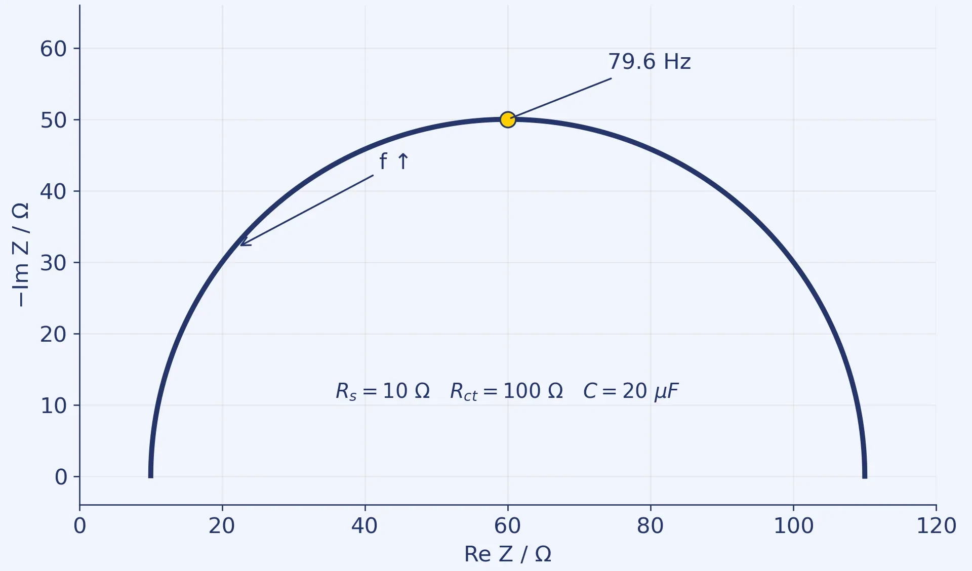
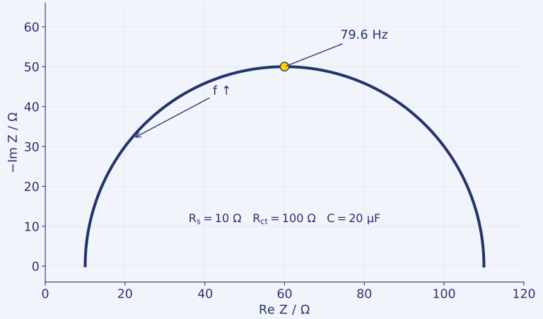
Consider Rₛ + (Rct ∥ C): a series resistor followed by a parallel resistor and ideal capacitor. Choose Rₛ = 10 Ω, Rct = 100 Ω and C = 20 µF. This is a teaching model without diffusion, inductance or surface heterogeneity.
Its impedance is:
Z(ω) = Rₛ + Rct / (1 + jωRctC), where j² = −1.
The equation directly gives the following results:
- At high frequency, Z approaches the 10 Ω series resistance.
- At low frequency, Z approaches the sum of the resistances: 110 Ω.
- The semicircle diameter is 100 Ω. Its apex is at Re Z = 60 Ω and −Im Z = 50 Ω.
- The time constant is τ = RctC = 0.002 s; the apex frequency is f = 1/(2πτ) ≈ 79.6 Hz.
At the apex, Z = 60 − j50 Ω, |Z| ≈ 78.1 Ω and the phase is approximately −39.8°. In this circuit, the Nyquist semicircle apex does not mean a total impedance phase of −45°: the series resistance also contributes to the real component.
Download the vector figure (SVG). The curve is calculated from the equation above, not measured. A similar shape from a real sample does not establish the same physical model. The label Rct denotes charge-transfer resistance only when an appropriate electrode-process model supports that interpretation.

Potential or current control?
PEIS modulates potential and measures current; GEIS does the reverse. Current control can be useful for low-impedance cells. GEIS-AA adjusts current excitation to target a voltage amplitude. Selecting a control mode does not itself make a sample stationary. BioLogic: PEIS, GEIS and GEIS-AA.
Our sizing example: a 10 mV amplitude across an impedance magnitude of 5 mΩ requires a 2 A current amplitude. Small voltage excitation need not mean a small current load. Both the DC operating point and AC excursion must remain within instrument and cell limits. Keep peak, peak-to-peak and RMS amplitude definitions distinct.
Before fitting a model
EC-Lab quality indicators address different issues: THD describes harmonic distortion, NSD time variation, and NSR noise relative to signal. The 5% threshold discussed by BioLogic is a guideline, not a universal acceptance criterion. Evaluate amplitude and usable frequency range together. BioLogic: reliable EIS measurements.
Calculate measurement time too: at 10 mHz, one period takes 100 seconds. Three periods take five minutes before settling time or other frequency points are included. Even a seemingly short frequency list can represent a long experiment.
Our EIS data-quality guide explains the calculation and checking sequence in more detail.
What should the measurement record contain?
This editorial checklist is a starting point for reproducibility:
- Sample identifier, cell configuration, electrodes and reference.
- Temperature, operating point and, for batteries, state of charge and pretreatment.
- PEIS/GEIS mode, amplitude and its definition, frequency limits.
- Point density, period count, waiting times and measurement ranges.
- Cabling, instrument configuration and software version.
- Raw data, quality indicators, excluded points and reasons for exclusion.
- Fitting model, weighting, parameter uncertainty and residuals.
Where to start with instrument selection
Use the instrument finder to summarise your requirements. Starting points for comparison include the SP-150e, SP-300 and, for battery work, the BCS-900 family. Their pages explain configuration limits and options; this list is not a personalised recommendation.
Include the expected impedance range and desired measurement time in the discussion. EC-Lab and the manufacturer application notes support more detailed method planning.